Solution: Cox-regression in R for Pneumonia data

Eksempel

Here we solve the problem linking to this page.

Solution to (a)

From the Cox-regression model \((1.32)\) we have

\[\alpha_i(t) = \alpha_0(t)e^{\beta x_i(t)},\]

so for a patient with pneumonia status \(x\) the hazard rate is

\[\alpha(t|x) = \alpha_0(t)e^{\beta x}.\]

Solution to (b)

We get that the partial likelihood in \((4.7)\) becomes:

\[L(\beta) = \prod_{T_j} \frac{\exp(\beta x_{i_j})}{\sum_{l \in R_j}\exp(\beta x_l)},\]

where \(i_j\) is the index of the individual with event time \(T_j\) and \(R_j = \{l: T_l \geq T_j\}\) are the indices of individuals still at risk right before \(T_j\). We can also calculate the partial log-likelihood:

\[l(\beta) = \sum_{T_j} \exp(\beta x_{i_j}) - \sum_{T_j}\sum_{l \in R_j}\exp(\beta x_l).\]

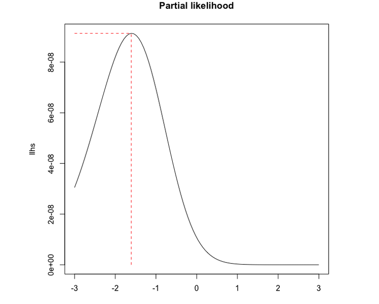
Code 1 shows R-code that calculates and plots the partial likelihood as a function of \(\beta\). NB: If you are refused access to the dataset through R, you may open the link in a web-browser and download the txt-file to your own computer.

Kopier

library(survival)
pneu=read.table("http://www.math.ntnu.no/emner/TMA4275/2021v/Datasets/pneumonia.txt",header=T)

#Order data by event times
order = order(pneu$time)
pneu$time = pneu$time[order]
pneu$x = pneu$x[order]
pneu$cens = pneu$cens[order]

#Make a function to calculate the partial likelihood for a given beta
partial_lh = function(beta){
  expbetas = exp(beta*pneu$x)
  
  n = length(expbetas)
  prod = 1
  for (i in 1:n){ #Product over all events
    if (pneu$cens[i]){ #Censored observations are left out
      numerator = expbetas[i]
      r = min(which(pneu$time == pneu$time[i]))
      #We need to be careful about the risk set when there are ties
      denominator = sum(expbetas[r:n])
      prod = prod*numerator/denominator
    }
  }
  return(prod)
}

betas = seq(-3,3,length.out = 100)
lhs = array(0,100)
for (i in 1:100){
  lhs[i] = partial_lh(betas[i])
}

plot(betas,lhs,type="l")
k = which.max(lhs)
lines(c(betas[1],betas[k]),c(lhs[k],lhs[k]),lty=2,col="red")
lines(c(betas[k],betas[k]),c(0,lhs[k]),lty=2,col="red")

Code 1: Code for plotting the partial likelihood of the Cox-regression model.

Figure 1 shows the resulting plot, and we can see that the maximum likelihood estimate of \(\beta\) is \[\hat \beta = -1.6.\]

Partial likelihood of Cox Model — Figure 1: Partial likelihood of a Cox-regression model. The value of \(\beta\) maximizing the likelihood is marked by the dashed, red line.

Solution to (c)

Running the provided code,

Kopier

fit.pneu = coxph(Surv(time,cens==1)~x,method="breslow",data=pneu)
summary(fit.pneu)

gives the output:

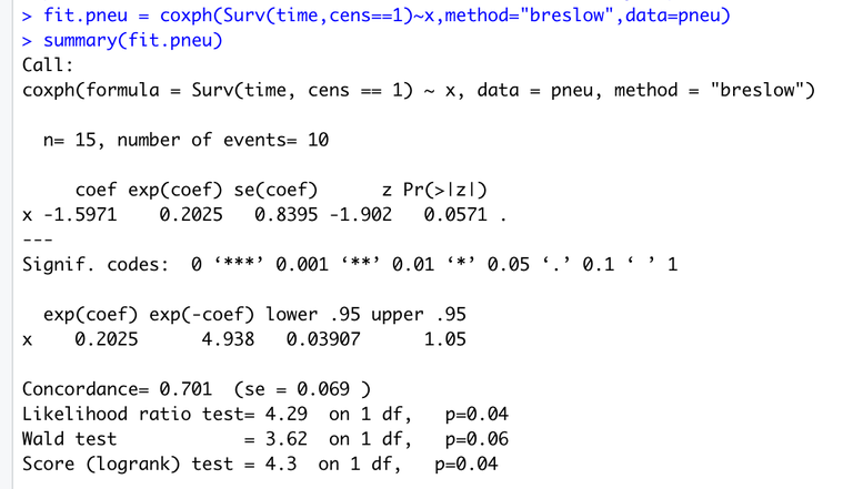
Coxfitsummary — Figure 2: Summary from fit of Cox model.

The estimate for \(\beta\) is read out under "coef", next to "x". Thus the estimate is \(\hat \beta = -1.5971\), corresponding to what we found above.

Solution to (d)

We want to test the hypothesis \[H_0: \beta = 0 \quad \text{vs.} \quad H_1: \beta \neq 0.\]

Using a significance level of \(5\%\), and the results of the score test in the summary above, we can conclude that there is a significant difference between the discharge times for patients without and with pneumonia (note that the Wald test does not yield a significant result, and that in an actual experiment the choice of test would be done before seeing the results of the tests).

The relative risk of a patient without pneumonia compared to a patient with pneumonia is

\[e^{\beta\cdot 1}/e^{\beta \cdot 0} = e^{\beta} = 0.2025,\]

meaning that a the rate of disharge for a patient with pneumonia at admission is a fifth of the rate for a patient without pneumonia.

Solution to (e)

The log-rank test tests a more general hypothesis that the two groups have the same hazard rate at all times, i .e. \[H_0: \alpha_1(t) = \alpha_2(t)\] for all \(t \in [0,t_0]\), where the hazard rates need not be specified. The tests above, on the other hand, test if the hazard rates are the same under the restriction of the Cox-regression model.

R-code for performing the log-rank test "by hand", as described in section 3.3.1 in ABG, is provided in Code 2 below (note that the dataset has been rewritten in a slightly different form):

Kopier

Times = c( 2, 3, 4, 6, 9,10,11,12,17,23,24,26,32) #Times of interest (events and censored observations)
d_P =   c( 0, 0, 0, 0, 1, 0, 0, 0, 1, 0, 1, 0, 1) #Number of events, Pneumonia
c_P =   c( 0, 0, 1, 0, 0, 0, 0, 1, 0, 0, 0, 1, 0) #Number of censored obs, Pneu
d_M =   c( 1, 0, 0, 2, 0, 1, 1, 0, 0, 1, 0, 0, 0) #Number of events, no pneu
c_M =   c( 0, 1, 0, 0, 0, 0, 0, 1, 0, 0, 0, 0, 0) #Number of censored obs, no pneu

d = d_P + d_M
c = c_P + c_M

#Number of individuals in each group
numP = 7 
numM = 8

m = length(Times)

#Calculate the number at risk at each time
Y_P = rep(numP,m)
Y_M = rep(numM,m)
Y_P[2:m] = Y_P[2:m] - cumsum(d_P+c_P)[1:(m-1)]
Y_M[2:m] = Y_M[2:m] - cumsum(d_M+c_M)[1:(m-1)]
Y = Y_P + Y_M

#Calculate the test statistic
Z_1 = sum(d_P*Y_M/Y - d_M*Y_P/Y)
V_11 = sum(d*Y_M*Y_P/Y^2)
X = Z_1^2/V_11

#Get the p-value
pchisq(X,1,lower.tail = F)

#Checking the expected values for each group
E_P = sum(d*Y_P/Y) #Expected number of observations in the Pneumonia group
E_M = sum(d*Y_M/Y) #Expected number of observations in the other group

Code 2: Performing the log-rank test for the hazard functions of the two patient groups.

This results in a p-value of 0.038, meaning the hypothesis that the hazard functions are equal is rejected.

Solution to (f)

Running the command

Kopier

survdiff(Surv(time,cens)~x,data=pneu)

gives the output:

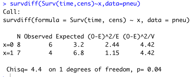
logrankreadout — Figure 3: Printout from log-rank test.

Hence we reach the same conclusion as we did in (d) (note that the test performed in R uses a slightly different estimate for the variance of \(Z_1\) than we did in (e), hence the slight difference in test statistic and p-value).