Solution: Competing risks model
Eksempel
Here we solve the problem linking to this page.
Solution to (a)
Let us first consider the case \(D = 1\), which means \(T_1 \leq T_2\). This means \(T = \min\{T_1,T_2\} = T_1\), so that:
\begin{align*} P(T \leq t, D=1) &= P(T_1 \leq t, T_1 \leq T_2) \end{align*}
We want to express this as an integral of the joint density of \(T_1\) and \(T_2\). In the \((T_1,T_2)\)-plane this is the area which has first coordinate smaller than or equal to \(t\), and second coordinate greater than or equal to the first coordinate. Note that \(T_1\) and \(T_2\) are independent, so that the joint density is \[f(t_1,t_2) = f_{T_1}(t_1)f_{T_2}(t_2).\]
Note also that the cumulative density function of \(T_j\) is \(F_{T_j}(t) = \int_0^t f_{T_j}(u)du =\int_0^t \lambda_j e^{-\lambda_j u}du = 1 - e^{-\lambda_j t}\). We now get
\begin{align*} P(T_1 \leq t, T_1 \leq T_2) &= \int_0^t \int_{t_1}^{\infty} f(t_1,t_2)dt_2dt_1 \\ &= \int_0^t \int_{t_1}^{\infty} f_{T_1}(t_1)f_{T_2}(t_2)dt_2dt_1 \\ &= \int_0^t \left[\int_{t_1}^{\infty}f_{T_2}(t_2)dt_2 \right]f_{T_1}(t_1)dt_1 \\ &= \int_0^t (1-F_{T_2}(t_1))f_{T_1}(t_1)dt_1 \\ &= \int_0^t e^{-\lambda_2 t_1}\lambda_1 e^{-\lambda_1 t_1}dt_1 \\ &= \int_0^t \lambda_1 e^{-(\lambda_1+\lambda_2) t_1}dt_1 \\ &= \frac{\lambda_1}{\lambda_1+\lambda_2}\left(1-e^{-(\lambda_1+\lambda_2) t}\right).\end{align*}
For the case \(D=2\) it is easy to see that interchanging the indices in the above argument yields the corresponding result, and thus that
\[\underline{\underline{P(T \leq t, D=j) = \frac{\lambda_j}{\lambda_1+\lambda_2}\left(1-e^{-(\lambda_1+\lambda_2) t}\right).}}\]
Solution to (b)
For the cause-specific hazard rate \(\alpha_j(t)\), we have that \(\alpha_j(t)dt\) is the probability of an event of cause \(j\) in an infinitesimal interval \([t,t+dt)\) given that the event has not occurred before \(t\). Using the limit definition of the hazard rate we get:
\begin{align*}\alpha_j(t) &= \lim_{\Delta t \rightarrow 0} \frac{1}{\Delta t} P(t \leq T < t + \Delta t, D=j | T \geq t),\end{align*}
where we can write
\begin{align*}P(t \leq T < t + \Delta t, D=j | T \geq t)&= \frac{P(t \leq T < t + \Delta t, D=j)}{P(T \geq t)} \\ &= \frac{P(T \leq t + \Delta t, D=j)-P(T \leq t , D=j)}{P(\min\{T_1,T_2\} \geq t)} \\ &= \frac{\frac{\lambda_j}{\lambda_1+\lambda_2}\left(1-e^{-(\lambda_1+\lambda_2) (t+\Delta t)}\right)-\frac{\lambda_j}{\lambda_1+\lambda_2}\left(1-e^{-(\lambda_1+\lambda_2) t}\right)}{P(T_1 \geq t, T_2 \geq t)} \\ &= \frac{\frac{\lambda_j}{\lambda_1+\lambda_2}e^{-(\lambda_1+\lambda_2) t}\left(1-e^{-(\lambda_1+\lambda_2) \Delta t}\right)}{P(T_1 \geq t, T_2 \geq t)} \\ &= \frac{\frac{\lambda_j}{\lambda_1+\lambda_2}e^{-(\lambda_1+\lambda_2) t}\left(1-e^{-(\lambda_1+\lambda_2) \Delta t}\right)}{(1-F_{T_1}(t))(1-F_{T_2}(t))} \\ &= \frac{\frac{\lambda_j}{\lambda_1+\lambda_2}e^{-(\lambda_1+\lambda_2) t}\left(1-e^{-(\lambda_1+\lambda_2) \Delta t}\right)}{e^{-\lambda_1 t}e^{-\lambda_2 t}} \\ &= \frac{\lambda_j}{\lambda_1+\lambda_2}\left(1-e^{-(\lambda_1+\lambda_2) \Delta t}\right) .\end{align*}
Now we can calculate the limit
\begin{align*}\alpha_j(t) &= \lim_{\Delta t \rightarrow 0} \frac{1}{\Delta t} \frac{\lambda_j}{\lambda_1+\lambda_2}\left(1-e^{-(\lambda_1+\lambda_2) \Delta t}\right) \\ &= \frac{\lambda_j}{\lambda_1+\lambda_2}\left(\lim_{\Delta t \rightarrow 0} \frac{1-e^{-(\lambda_1+\lambda_2) \Delta t}}{\Delta t}\right) \quad \left(\text{0/0-expression}\right) \\ &= \frac{\lambda_j}{\lambda_1+\lambda_2}\left(\lim_{\Delta t \rightarrow 0} \frac{\frac{d}{d\Delta t}\left(1-e^{-(\lambda_1+\lambda_2) \Delta t}\right)}{\frac{d}{d\Delta t}\Delta t}\right) \\ &= \frac{\lambda_j}{\lambda_1+\lambda_2}\left(\lim_{\Delta t \rightarrow 0} \frac{(\lambda_1+\lambda_2)e^{-(\lambda_1+\lambda_2) \Delta t}}{1}\right) \\ &= \frac{\lambda_j}{\lambda_1+\lambda_2}\left(\lambda_1+\lambda_2\right) \\ &= \lambda_j .\end{align*}
Solution to (c)
The cause-specific hazard rate is the instantaneous rate of occurrence a given type of event in an individual conditioned on that individual surviving until that point in time, and is thus independent of the other types of events. The cumulative incidence function, on the other hand, is the probability of an event of a given type occurring first, which requires the other types of events to not have happened, and must necessarily depend on the distribution of these.
Solution to (d)
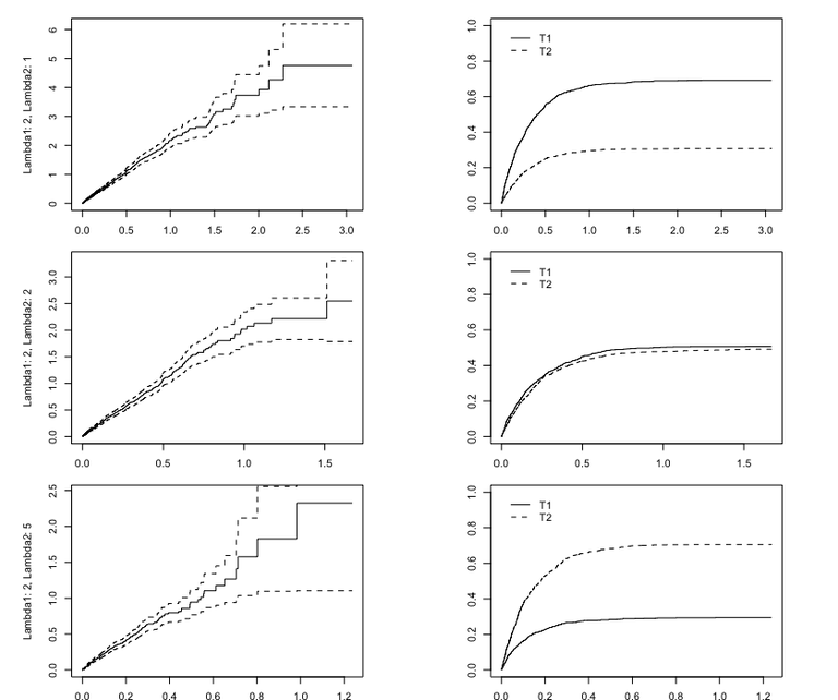
In the code below we simulate data for selected values of \(\lambda_1\) and \(\lambda_2\), and plot the estimated cause-specific cumulative hazard rate for \(T_1\) and the cumulative incidence functions for \(T_1\) and \(T_2\).
library(survival)
library(cmprsk)

#Number of simulations
nsim <- 1000

simulate_and_plot = function(nsim,lambda1,lambda2,seed){
  #Simulate data
  set.seed(seed)
  T1s <- rexp(nsim,lambda1)
  T2s <- rexp(nsim,lambda2)

  obstime <- array(0,nsim)
  obstime <- pmin(T1s,T2s)
  d <- 1*(obstime==T1s)+2*(obstime==T2s)

  causespec1 <- survfit(Surv(obstime,d==1)~1,type="fh2")
  plot(causespec1,fun="cumhaz",mark.time=F,
       ylab=paste("Lambda1: ",lambda1,", Lambda2: ",lambda2,sep=""),ylim=c(0,lambda1*max(causespec1$time)))

  #Estimate and plot the cimulative incidence functions:
  ci = cuminc(obstime,d)
  plot(ci$`1 1`$time,ci$`1 1`$est,lty=1,type="s",ylim=c(0,1),ylab="")
  lines(ci$`1 2`$time,ci$`1 2`$est,lty=2,type="s",ylab="")
  legend(0,1,c("T1","T2"),lty=1:2,bty="n")
}

par(mfrow=c(3,2))
simulate_and_plot(nsim,lambda1=2,lambda2=1,seed=4275)
simulate_and_plot(nsim,lambda1=2,lambda2=2,seed=4275)
simulate_and_plot(nsim,lambda1=2,lambda2=5,seed=4275)
Figure 1 shows the resulting plots. Notice that the estimates for the cause-specific cumulative hazard rate for \(T_1\) (left plots) does not change particularly much when varying \(\lambda_2\). The confidence bounds widen, because an increase in \(\lambda_2\) makes it more likely that \(T_2 < T_1\), which means there will be fewer observations of \(T_1\).
The estimates for the cumulative incidence functions do change, as expected, and we see that as \(\lambda_2\) increases relatively to \(\lambda_1\), the cumulative incidence function for \(T_1\) is reduced.