Solution: Cox-regression, martingale residuals and transformations
Eksempel
Here we solve the problem linking to this page, using the provided code and discussing in light of the properties found in section 4.1.3 in ABG, as well as the video in Model checking in Cox regression.
Solution to (a)
The \(x\) are drawn from a Gamma-distribution with shape parameter \(\alpha = 2\) and rate parameter \(\beta = 1\) (default value, since it is not specified). Thus the density is
\[f_X(x) = \frac{1^2}{\Gamma(2)}x^{2-1}e^{-1\cdot x} = xe^{-x}.\]
The \(C\) are drawn from an Exponential-distribution with rate parameter \(\lambda = 0.5\), and so the density is
\[f_C(c) = 0.5 e^{-0.5 c}.\]
The hazard rate can be found through the relation \(\alpha(t) = \frac{-S'(t)}{S(t)}\), where \(S(t) = P(T > t)\) is the survival function of \(T\). We have \(T = \sqrt{2Ue^{-x}}\) where \(U\) has an exponential distribution with rate parameter \(\lambda = 1\), so that \(F_U(u) = 1 - e^{-x}\). Thus
\begin{align*} S(t) &= P(T > t) \\ &= P( \sqrt{2Ue^{-x}} > t) \\ &= P( 2Ue^{-x} > t^2) \\ &= P(U > \frac{1}{2}t^2e^x) \\ &= 1 - F_U(\frac{1}{2}t^2e^x) \\ &= \exp\left(-\frac{1}{2}t^2e^x\right) ,\end{align*}
and so \[S'(t) = -te^x\exp\left(-\frac{1}{2}t^2e^x\right),\]
and \[\alpha(t) = te^x.\]
Solution to (b)
Running the provided code yields the output
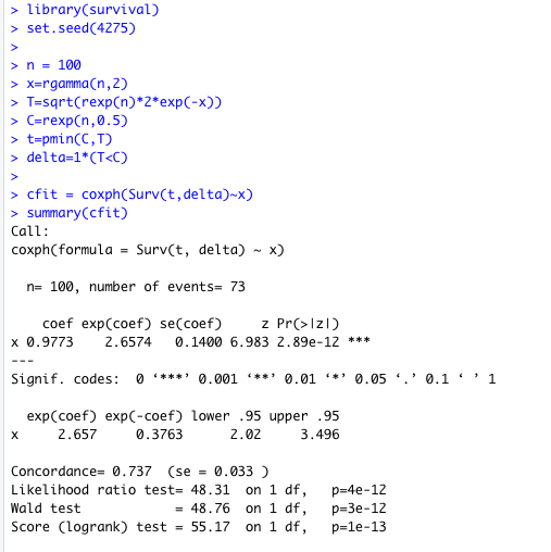
Note that we fit the model \(\alpha(t|x) = \alpha_0(t)e^{\beta x}\), where we know the truth to be \(\alpha_0(t) = t\) and \(\beta=1\) (keep in mind that we only estimate the relative risk, and not \(\alpha_0\)). The output seems to correspond well with this.
Figure 2 shows the martingale residuals with the lowess smooth.
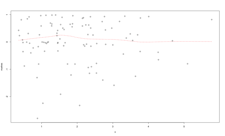
The residuals seem to be distributed with mean 0, which is what we expect.
Solution to (c)
Now we have \(T = \sqrt{2Ue^{-\log(x)}}\), where \(U\) has the same distribution as before. Thus we get
\[S(t) = \exp\left(-\frac{1}{2}t^2e^{\log(x)}\right),\]
\[S'(t) = -te^{\log(x)}\exp\left(-\frac{1}{2}t^2e^{\log(x)}\right),\]
and
\[\alpha(t) = te^{\log(x)} = tx.\]
The Cox model we are fitting is thus \(\alpha(t|x) = \alpha_0(t)e^{\beta \log(x)}\), where the transformation of \(x\) is \(f(x) = \log(x)\).
Solution to (d)
Fitting the slightly wrong model yields output
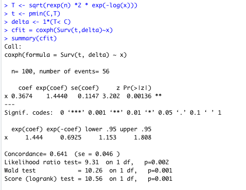
We can see that we still get a significant result, but the fit seems worse than before. Figure 4 shows the martingale residuals and lowess smooth.
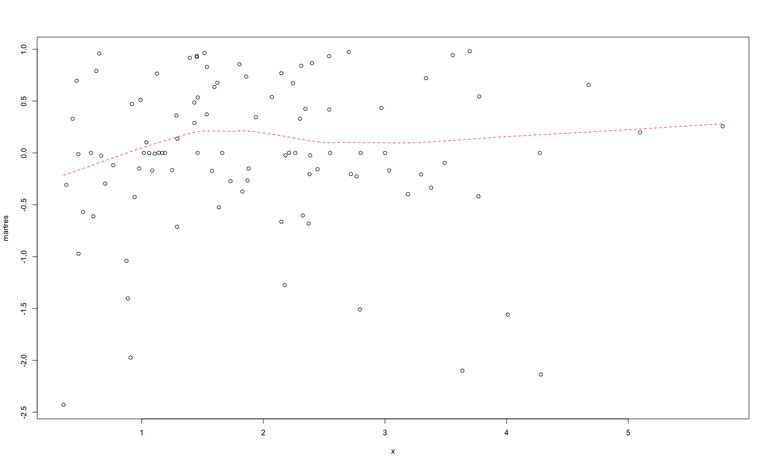
Here there seems to be a slight trend where the mean of the residuals deviates from 0, suggesting that the fit is imperfect.
Solution to (e)
We fit models using the transformations \(f(x) = x\), \(f(x) = x^ 2\), \(f(x) = \log(x)\) and \(f(x) = \sqrt{x}\). Code 1 shows how you can fit these models and plot the respective martingale residuals in R:
x2 = x^2
cfitx = coxph(Surv(t,delta)~x)
cfitx2 = coxph(Surv(t,delta)~x2)
cfitlogx = coxph(Surv(t,delta)~log(x))
cfitsqrtx = coxph(Surv(t,delta)~sqrt(x))

martresx = cfitx$residuals
martresx2 = cfitx2$residuals
martreslogx = cfitlogx$residuals
martressqrtx = cfitsqrtx$residuals

par(mfrow=c(1,1))
plot(x,martresx)
lines(lowess(x,martresx),col="black",lty=2,lwd=2)
points(x,martresx2,col="red")
lines(lowess(x,martresx2),col="red",lty=2,lwd=2)
points(x,martreslogx,col="green")
lines(lowess(x,martreslogx),col="green",lty=2,lwd=2)
points(x,martressqrtx,col="blue")
lines(lowess(x,martressqrtx),col="blue",lty=2,lwd=2)
legend(5,-1.5,c("f(x) = x","f(x) = x^2","f(x) = log(x)","f(x) = sqrt(x)"),col=c("black","red","green","blue"),lty=2,lwd=2)
The resulting residuals are plotted together in Figure 5.
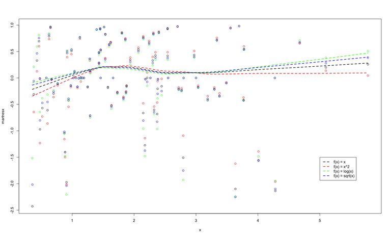
Although it is not very clear, the transformation \(f(x) = \log(x)\) (which is the true transformation) appears to have residuals with a mean that is slightly more consistent along 0.