Solution: Kaplan-Meier estimator for Leukemia data

Eksempel

Here we solve problem 3.7 in ABG, using the definition in section 3.2.1 and the modifications needed to handle ties from section 3.2.2.

Solution to (a)

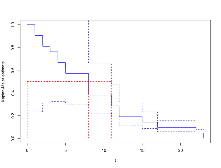
The Kaplan-Meier estimator for the survival function \(S(t)\) (\((3.26)\) in ABG) is given by \[\hat S(t) = \prod_{T_j \leq t} \left\{1-\frac{1}{Y(T_j)}\right\},\] where \(Y(t)\) is the number of individuals at risk just before time \(t\) and \(0 < T_1 < \ldots\) are the event times. Here we have ties, since the remission time is rounded to whole weeks. We therefore adjust the estimates using the correction \((3.32)\) in ABG, given by \[\hat S(t) = \prod_{T_j \leq t} \left\{1-\frac{d_j}{Y(T_j)}\right\},\] where \(d_j\) is the number of events happening at time \(T_j\).

For the placebo group we have

LeukemiaPlacebo — Table 1: Data for the placebo group, with event times in the top row, number at risk just before the event times in the middle row, and the number of events at each event time in the bottom row.

Code 1 contains some R code that calculates and plots the Kaplan-Meier estimate for the placebo group according to the formula stated above, with confidence limits from \((3.30)\).

Kopier

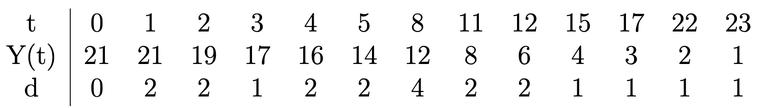
Times = c(0,1,2,3,4,5,8,11,12,15,17,22,23) #Event times
d = c(0,2,2,1,2,2,4,2,2,1,1,1,1) #Number of events
c = rep(0,length(Times)) #Censored observations

Kaplan_Meier = function(Times,d,c){
  # Calculates the Kaplan-Meier estimate according to 3.32 in ABG
  m = length(Times)
  Y = rep(21,m)
  Y[2:m] = Y[2:m] - cumsum(d+c)[1:(m-1)]
  
  S = cumprod(1 - d/Y)
  
  Shat = stepfun(Times[2:m],S)
  
  return(Shat)
}

SigmaHat2 = function(Times,d,c){
  # Calculates the variance estimate in 3.14/3.15,
  # which will then be used to calculate the estimated variance
  # of the Kaplan-Meier estimates
  m = length(Times)
  Y = rep(21,m)
  Y[2:m] = Y[2:m] - cumsum(d+c)[1:(m-1)]
  
  Deltahatsigma2 = rep(0,m)
  for (j in 1:m){
    # This is the adjusted inner sum
    if (d[j] > 0){
      for (l in 0:(d[j]-1)){
        Deltahatsigma2[j] = Deltahatsigma2[j] + 1/(Y[j]-l)^2
      }
    }
  }
  hatsigma2 = stepfun(Times[2:m],cumsum(Deltahatsigma2))
  
  return(hatsigma2)
}

hatS = Kaplan_Meier(Times,d,c)

t = seq(0,max(Times),by=0.01)

hatTau2 = hatS(t)^2*SigmaHat2(Times,d,c)(t)
exponent = qnorm(0.975)*sqrt(hatTau2)/(hatS(t)*log(hatS(t)))
conf_upper = hatS(t)*exp(-exponent)
conf_lower = hatS(t)*exp(exponent)

par(mfrow = c(1,1))
plot(t,hatS(t),type="l",col="blue",ylab="Kaplan-Meier estimate")
lines(t,conf_upper,lty=2,col="blue")
lines(t,conf_lower,lty=2,col="blue")

Code 1: Calculating and plotting the Kaplan-Meier estimate and confidence limits for the Placebo group in the Leukemia data.

Figure 1 shows the resulting plot:

KaplanMeierLeukemia — Figure 1: The resulting plot from Code 1, showing the Kaplan-Meier estimate with \(95\%\) confidence limits for the placebo group.

Solution to (b)

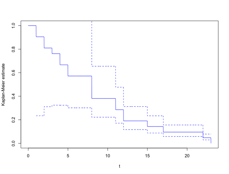
We use the method described in section 3.2.3 to find an estimate and a \(95\%\) confidence interval for the median relapse time for the placebo group. From the plot in figure 1 we see that the estimate jumps below 0.5 at \(t=8\), and hence our estimate is \(\hat \xi_{0.5} = 8\). For the confidence interval, first observe that the lower confidence bound for the Kaplan-Meier estimate is always smaller than 0.5, and so the lower bound for our confidence interval for the median relapse time is 0. The upper confidence bound jumps below 0.5 at \(t=11\), and hence our confidence interval is \([0,11]\). Figure 2 illustrates this:

KaplanMeierLeukemiaMedian — Figure 2: Using the confidence bounds for the Kaplan-Meier estimate, we can find an estimate and a confidence interval for the median relapse time.