Solution: Survival function and density for the Weibull distribution

Eksempel

We start by finding the survival function \(S(t)\) from the given hazard rate \(\alpha(t),\) and thereafter find the density \(f(t)\) from the survial function \(S(t).\)

Survival function

The survival function \(S(t)\) is given from the hazard rate \(\alpha (t)\) by \[S(t)=\exp\left\{-\int_{0}^{t}\alpha(s)ds\right\}.\] With hazard rate \(\alpha(t) = bt^{k-1}, t > 0\) we thus get \begin{align*}S(t) &= \exp\left\{-\int_{0}^{t}bs^{k-1}ds\right\} \\ &= \exp\left\{-\left(\frac{b}{k}t^k-\frac{b}{k}0^k\right)\right\} \\ &= \exp \left(-\frac{bt^k}{k}\right).\end{align*} Thus, the survival function for the Weibull distribution is \[\underline{\underline{S(t)=\exp \left(-\frac{bt^k}{k}\right),t>0.}}\]

Density

The survival function \(S(t)\) is defined as \[S(t)=P(T>t),\] and the density of \(T\) can thus be found through the cumulative distribution of \(T\), since \[f(t) = \frac{d}{dt}F(t)\] and \[F(t) = P(T \leq t) = 1 - P(T > t).\] When the survival function is as given above we get \begin{align*} f(t) &= \frac{d}{dt} F(t) \\ &= -\frac{d}{dt}S(t) \\ &= -\frac{d}{dt}\exp \left(-\frac{bt^k}{k}\right) \\ &= -\exp \left(-\frac{bt^k}{k}\right)\frac{d}{dt}\left(-\frac{bt^k}{k}\right) \\&= bt^{k-1}\exp \left(-\frac{bt^k}{k}\right)\end{align*} Thus the density for the Weibull distribution is \[\underline{\underline{f(t)= bt^{k-1}\exp \left(-\frac{bt^k}{k}\right),t>0.}}\]

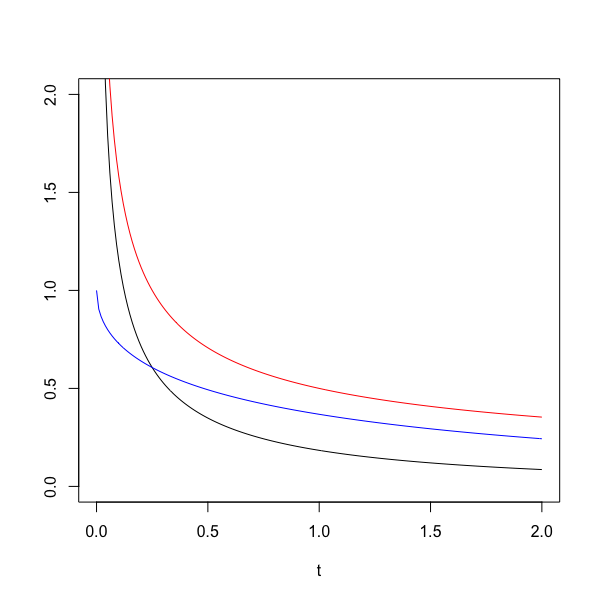
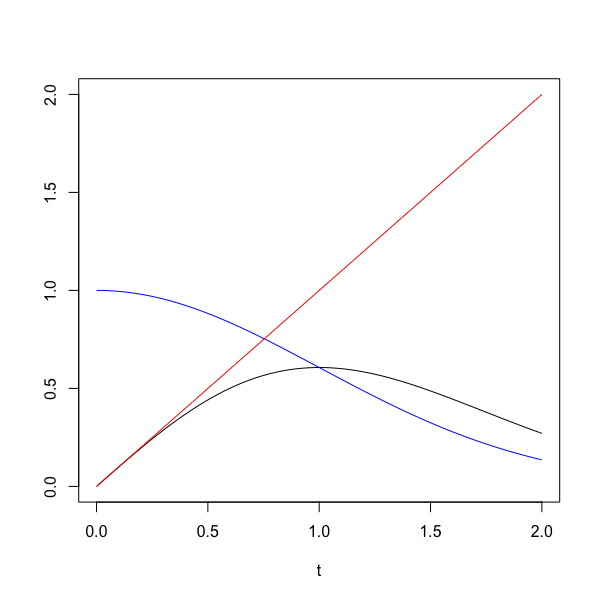
Plots of \(f(t),\) \(S(t)\) and \(\alpha(t)\) for \(b = 1, k = 2\) and \(b = k = \frac{1}{2}\)

The R code in Code 1 can be used to plot the density function, survival function and the hazard rate when \(b = 1\) and \(k = 2\) on the interval \(t\in (0,2).\)

Kopier

b = 1.0
k = 2.0
t = seq(0,2,0.01)
plot(t,b*t^(k-1)*exp(-b*t^k/k),col="black",xlab="t",ylab="",type="l")
lines(t,exp(-b*t^k/k),col="blue",type="l")
lines(t,b*t^(k-1),col="red",type="l")

Code 1: R code for plotting density function, survival function and hazard rate of the Weibull distribution. The density function is black, the survival function is blue and the hazard rate is red.

Figure 1 shows the plot that is produced by running the R code in Code 1.

Figure 1: The density function (in black), the survival function (in blue) and the hazard rate (in red) for a Weibull distribution with parameters \(b=1\) and \(k=2./) — Figure 1: The density function (in black), the survival function (in blue) and the hazard rate (in red) for a Weibull distribution with parameters \(b=1\) and \(k=2.\)

The R code in Code 1 can be modified to plot the density function, survival function and the hazard rate when \(b = k = 0.5\) on the interval \(t\in (0,2),\) by changing the values that \(b\) and \(k\) are set to. Figure 2 shows the plot that is produced by running the R code in Code 1 with these adjustments.

Figure 2: The density function (in black), the survival function (in blue) and the hazard rate (in red) for a Weibull distribution with parameters \(b=k=0.5.\)