Solution: Interpretation of survival curves

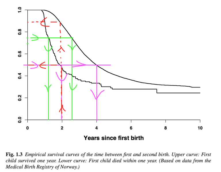
Figure 1.3 in ABG shows the empirical survival function for each of the two groups. This means that the curve is an estimate of \(S(t) = P(T > t)\), and 1 minus the curve is an estimate of \(P(T \leq t)\). We are interested in the probability of having another child within two years of the birth of the first child, and thus the probability \(P(T \leq 2)\). Finding the values on the curves corresponding to \(t=2\) yields and approximate probability of \(1-0.9 = 0.1\) for the women whose first child survived one year, and \(1-0.5 = 0.5\) for the women whose first child did not. See the figure at the bottom of this page for an illustration.

We are now interested in the lower quartile, meaning the value \(\xi_{0.25}\) for which \(P(T \leq \xi_{0.25}) = 0.25\), and the median\(\xi_{0.5}\) for which \(P(T \leq \xi_{0.5}) = 0.5\). Estimates of these can be found by looking at where each estimated survival function reaches \(1-0.25 = 0.75\) and \(1-0.5=0.5\), respectively.

The estimated survival function for women whose first child survived one year reaches the value \(0.75\) at approximately \(2.5\) years, which is thus an estimate of the lower quartile. It reaches \(0.5\) at approximately \(4\) years, which is thus an estimate of the median.

For the women whose first child did not survive one year the estimates are \(1.2\) years and \(2\) years, respectively.