Solution: Hazard rate and density function for the gamma distribution
Eksempel
Here we solve the slightly modified version of problem 1.1 (c) in ABG.
Solution
We have survival function \[S(t) = \frac{\Gamma(k,\gamma t)}{\Gamma(k)}, t>0,\] where \[\Gamma(k,x)= \int_x^\infty u^{k-1} e^{-u} du\] is the (upper) incomplete gamma function and \[\Gamma(k) = \int_0^\infty u^{k-1}e^{-u}du\] is the gamma function. We are to find the density function and hazard rate.
Density function
To find the density function we use that \(f(t) = \frac{d}{dt} F(t) = \frac{d}{dt} (1 - S(t))\), so that
\begin{align*} f(t) &= \frac{d}{dt} \left( 1 - \frac{\Gamma(k,\gamma t)}{\Gamma(k)}\right) \\ &= -\frac{\frac{d}{dt} \Gamma(k,\gamma t)}{\Gamma(k)}.\end{align*}
Using the fact that \(\frac{d}{dx} \int_x^{\infty} g(u)du = -g(x)\) (and the chain rule), we get that
\begin{align*} f(t) &= -\frac{\frac{d}{dt}\int_{\gamma t}^\infty u^{k-1} e^{-u} du}{\Gamma(k)} \\ &= -\frac{\frac{d}{d\gamma t}\int_{\gamma t}^\infty u^{k-1} e^{-u} du \cdot \gamma}{\Gamma(k)} \\ &= \frac{(\gamma t)^{k-1}e^{-\gamma t} \gamma}{\Gamma(k)} \\ &= \frac{\gamma^k}{\Gamma(k)} t^{k-1}e^{-\gamma t},\end{align*}
which one might recognize as the density of a gamma distribution with shape parameter \(k\) and rate parameter \(\gamma\).
Hazard rate
To find the density function we use that \(\alpha(t) = -\frac{d}{dt} \log S(t)\), so that
\begin{align*} \alpha(t) &= -\frac{d}{dt} \left( \log \Gamma(k,\gamma t) - \log \Gamma(k)\right) \\ &= -\frac{\frac{d}{dt} \Gamma(k,\gamma t)}{\Gamma(k,\gamma t)}.\end{align*}
This is very similar to the expression above, and we can easily see that we get
\[\alpha(t) = \frac{\gamma^k}{\Gamma(k,\gamma t)} t^{k-1}e^{-\gamma t}.\]
Plots in R
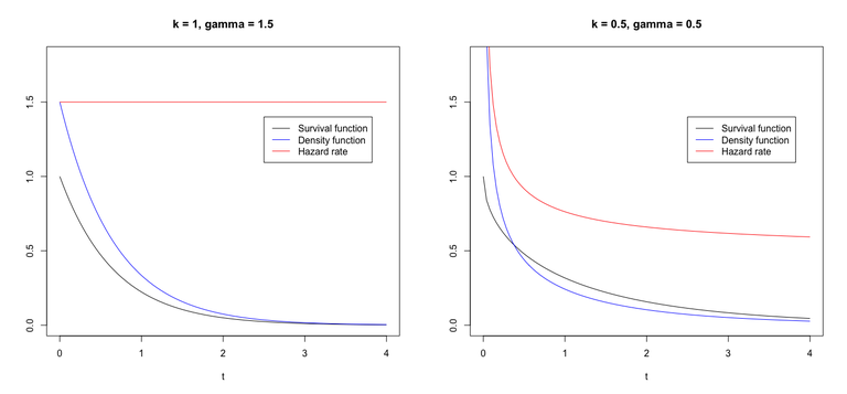
The code below can be used to plot the survival function, density function and hazard rate for the gamma distribution with \(k=1, \gamma=1.5\) and \(k=0.5, \gamma=0.5\). Note that the incomplete gamma function is calculated by using the cumulative distribution function. For more information about this use the command "?pgamma" in R.
n = 100
t = seq(0, 4, length.out = n)

gammas = c(1.5, 0.5)
ks = c(1, 0.5)

par(mfrow=c(1,2))
for (i in 1:2){
  k = ks[i]
  gamma = gammas[i]

  Gamma_k = gamma(k)
  Incomplete_gamma = pgamma(gamma*t,k,lower=FALSE)*Gamma_k
  #You can use the command "?pgamma" to find information about this way to calculate the incomplete gamma function

  S_t = Incomplete_gamma/Gamma_k
  f_t = gamma^k/Gamma_k*t^(k-1)*exp(-gamma*t)
  alpha_t = gamma^k/Incomplete_gamma*t^(k-1)*exp(-gamma*t)

  plot(t,S_t,type="l",ylim=c(0,1.8),ylab="",main=paste("k = ",k,", gamma = ",gamma,sep=""))
  lines(t,f_t,col="blue")
  lines(t,alpha_t,col="red")
  legend(2.5,1.4,legend=c("Survival function","Density function","Hazard rate"),col=c("black","blue","red"),lty=1)
}
The figure below shows the resulting plots. Note that for \(k=1\) the gamma distribution is equal to an exponential distribution, and the hazard rate is constant.