Solution: Finding fractiles from the integrated hazard rate
Eksempel
Here we solve exercise 1.2 in ABG, using the definitions from the book.
Solution to 1.2a)
The cumulative/integrated hazard rate is given by \(A(t) = \int_0^t\alpha(s)ds\), where we further have that the hazard rate \(\alpha(t)\) can be expressed using the cumulative distribution function of \(T\) through the relation \(\alpha(t) = -\frac{d}{dt}\log S(t) = -\frac{d}{dt}\log (1-F(t))\). Considering the fractile \(\xi_p\), defined so that \(F(\xi_p)=p\), we wish to show that \(A(t) = -\log(1-p)\) if and only if \(t = \xi_p\). Calculating the cumulative hazard rate by using the cumulative distribution function yields \begin{align*}A(t) &= \int_0^t\alpha(s)ds\\ &= \int_0^t-\frac{d}{ds}\log (1-F(s))ds \\ &= \int_0^t-\frac{\frac{d}{ds} (1-F(s))}{(1-F(s)}ds.\end{align*} We can simplify this expression by using the substitution \(u(s) = 1 - F(s)\), yielding limits \(u(0) = 1 - F(0) = 1 - 0 = 1\) and \(u(t) = 1 - F(t)\), which gives us \begin{align*}A(t) &= \int_0^t-\frac{\frac{d}{ds} (1-F(s))}{(1-F(s)}ds \\ &= \int_0^t-\frac{\frac{d}{ds} u(s)}{u(s)}ds \\ &= \int_{u(0)}^{u(t)}-\frac{1}{u}du \\ &= -\left(\log u(t) - \log u(0)\right) \\ &= -\left(\log (1-F(t)) - \log 1\right) \\ &= -\log \left(1-F(t)\right). \end{align*} Since \(\log\) is bijective, we get that \(A(t) = -\log(1-p)\) if and only if \(F(t) = p\), which, since \(F\) is assumed to be continuous and strictly increasing, happens if and only if \(t = \xi_p\).
Solution to 1.2b)
We use the relation \(F(t) = 1 - S(t)\) and solve the equation \(F(\xi_p) = p\) to find the expressions for \(\xi_p\) for the exponential distribution and the Weibull distribution.
Exponential distribution
With survival function \(S(t) = e^{-\lambda t}\) we get cumulative distribution function \(F(t) = 1 - e^{-\lambda t}\), and thus \begin{align*} F(\xi_p) &= 1 - e^{-\lambda \xi_p} = p \\ e^{-\lambda \xi_p} &= 1- p \end{align*} \[\underline{\underline{ \xi_p = \frac{-\log (1-p)}{\lambda}.}}\]
Weibull distribution
With survival function \(S(t) = \exp\left\{-\frac{bt^k}{k}\right\}\) we get cumulative distribution function \(F(t) = 1 - \exp\left\{-\frac{bt^k}{k}\right\}\), and thus \begin{align*} F(\xi_p) &= 1 - \exp\left\{-\frac{b\xi_p^k}{k}\right\} = p \\ \xi_p^k &= \frac{-k\log (1-p)}{b} \end{align*} \[\underline{\underline{ \xi_p = \left(\frac{-k\log (1-p)}{b}\right)^{\frac{1}{k}}.}}\]
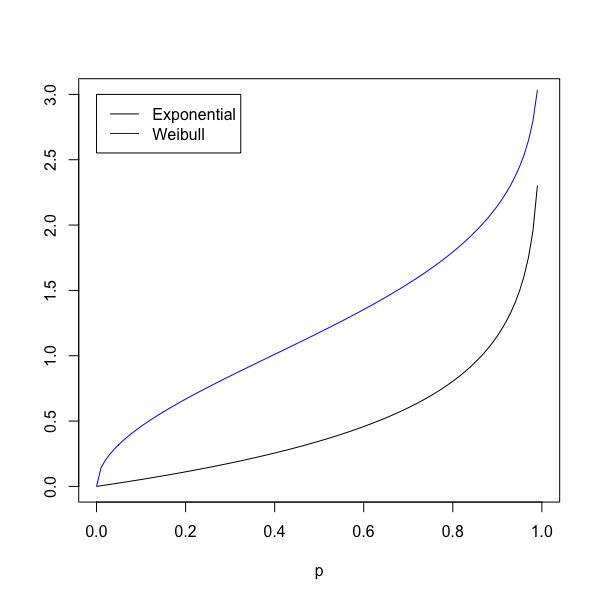
Plots of \(\xi_p\) for the exponential distribution with \(\lambda = 2.0\) and for the Weibull distribution with \(b = 1, k = 2\)
The R code in Code 1 can be used to plot the \(p\)th fractile \(\xi_p\) for the exponential distribution with \(\lambda = 2.0\) and for the Weibull distribution with \(b = 1\) and \(k = 2.\)
lambda = 2.0
b = 1
k = 2
p = seq(0,1,0.01)
plot(p,(-k*log(1-p)/b)^(1/k),col="blue",xlab="p",ylab="",type="l")
lines(p,-log(1-p)/lambda,col="black")
legend(0,3,c("Exponential","Weibull"),col=c("black","blue"),lty=1)
Figure 1 shows the plot that is produced by running the R code in Code 1.
