Solution: A simple counting process

Solution to 1.6a)

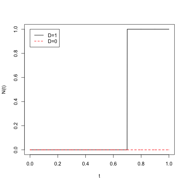
Our counting process \(N(t)\) is counting one potential event, effectively with right-censoring at \(t=1\). If \(D=0\), we do not observe the event, so we get \(N(t) = 0\) for \(t>0\). If \(D=1\) we will observe some \(\widetilde T \leq 1\), so that \(N(t) = 0\) for \(t < \widetilde T\) and \(N(t)=1\) for \(t \geq \widetilde T\). Code 1 shows how you can make a simple plot of this in R. Figure 1 shows the resulting plot.

Kopier

Ttilde = 0.7 #Arbitrarily chosen value for the sake of illustration
t = seq(0,1,by=0.001)
N = stepfun(Ttilde,c(0,1))
plot(t,N(t),type="l",lwd=1.5)
lines(t,0*t,col="red",lwd=1.5,lty=2)
legend(0,1,c("D=1","D=0"),col=c("black","red"),lty=c(1,2),lwd=1.3)

Code 1: Code for plotting \(N(t)\) for the cases \(D=0\) and \(D=1\) on the interval \(t \in (0,1)\).

Figure 1: Plot of \(N(t)\) for the cases \(D=0\) and \(D=1\) on the interval \(t \in (0,1)\).

Solution to 1.6b)

Using the definition of the intensity process (see section 1.4.2 in ABG), we have \[\lambda(t)dt = P(dN(t) = 1 \mid \text{past}) = P(t \leq \widetilde T < t + dt, D = 1 \mid \text{past}).\] Note that if \(\widetilde T < t\), so that the event has occurred before \(t\), the probability of it occurring later must necessarily be \(0\). By the independent censoring assumption and the definition of the hazard rate (section 1.1.2 in ABG) we get \begin{align*} \lambda(t)dt &= P(t \leq \widetilde T < t + dt, D = 1 \mid \text{past}) \\ &= I(\widetilde T \geq t) P(t \leq T < t + dt \mid T \geq t) \\ &= I(\widetilde T \geq t) \alpha(t)dt. \end{align*} Thus, with \(\alpha(t) = 2\) we get \[\underline{\underline{\lambda(t)=2I(\widetilde T \geq t) .}}\] In words we have \(\lambda(t) = 2\) for \(t < \widetilde T\), and \(0\) for larger \(t\). Thus the integrated intensity process \(\Lambda(t) = \int_0^t\lambda(s)ds\) is given by \(\Lambda(t) = 2t\) if \(t \leq \widetilde T\), and \(\Lambda(t) = 2\widetilde T\) if \(t > \widetilde T\).

Note: We could have applied the results from \((1.22)\) and \((1.23)\) in ABG directly in this problem. The derivation of the results is also shown in the video linked below.

Code 2 shows how you can make a simple plot of \(\Lambda(t)\) in R. Figure 2 shows the resulting plot.

Kopier

Ttilde = 0.7
alpha = 2
t = seq(0,1.5,by=0.001)
Lambda = function(t,Ttilde,alpha){
  y = array(0,dim=length(t))
  y[which(t <= Ttilde)] = t[which(t <= Ttilde)]*alpha
  y[which(t > Ttilde)] = alpha*Ttilde
  return(y)
}
plot(t,Lambda(t,Ttilde,alpha),type="l",lwd=1.5,ylab="",ylim=c(0,2.2))
lines(t,Lambda(t,1,alpha),col="red",lwd=1.5,lty=2)
legend(0,2,c("D=1","D=0"),col=c("black","red"),lty=c(1,2),lwd=1.3)

Code 2: Code for plotting \(\Lambda(t)\) for the cases \(D=0\) and \(D=1\) on the interval \(t \in (0,1.5)\).

Figure 2: Plot of \(\Lambda(t)\) for the cases \(D=0\) and \(D=1\) on the interval \(t \in (0,1.5)\).

Solution to 1.6.c)

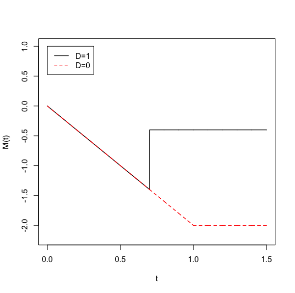
Combining our previous results we can find \(M(t) = N(t) - \Lambda(t)\). Code 3 shows how you can make a simple plot of this. Figure 3 shows the resulting plot.

Kopier

Ttilde = 0.7
alpha = 2
t = seq(0,1.5,by=0.001)
N = stepfun(Ttilde,c(0,1))

Lambda = function(t,Ttilde,alpha){
  y = array(0,dim=length(t))
  y[which(t <= Ttilde)] = t[which(t <= Ttilde)]*alpha
  y[which(t > Ttilde)] = alpha*Ttilde
  return(y)
}

M1 = N(t)-Lambda(t,Ttilde,alpha)
M0 = 0-Lambda(t,1,alpha)
plot(t,M1,type="l",lwd=1.5,ylab="M(t)",ylim=c(-2.2,1))
lines(t,M0,col="red",lwd=1.5,lty=2)
legend(0,1,c("D=1","D=0"),col=c("black","red"),lty=c(1,2),lwd=1.3)

Code 3: Code for plotting \(M(t)\) for the cases \(D=0\) and \(D=1\) on the interval \(t \in (0,1.5)\).

Figure 3: Plot of \(M(t)\) for the cases \(D=0\) and \(D=1\) on the interval \(t \in (0,1.5)\).