Solution: Simulating a Poisson process

Eksempel

Here we solve the problem linking to this page. We simulate the processes in R.

Solution

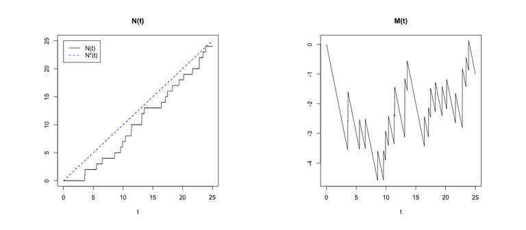
Recall that if \(N(t)\) is a homogeneous Poisson process with intensity \(\lambda\), the waiting times between events are independent and exponentially distributed with rate \(\lambda\). Thus, to simulate \(N(t)\) we can sample from the exponential distribution, adding the resulting waiting times together to find the event times. Code 1 shows a simple script that does this in R, and plots the sample path together with the compensator \(N^*(t)\) and also the corresponding path of \(M(t) = N(t) - N^*(t)\) in a separate plot.

Kopier

set.seed(4275)
lambda = 1
event_times = c()
latest = 0 #temporary variable to see if we're beyond the end of the interval
max_time = 25
while (latest <= max_time){
  # waiting times are independent and exponentially distributed
  new_waiting_time = rexp(n=1,rate=lambda)
  latest = latest+new_waiting_time
  event_times = c(event_times,latest)
}

t = seq(0,25,by=0.01)
N = stepfun(event_times,0:length(event_times))

par(mfrow=c(1,2))
plot(t,N(t),type="l",ylab="",ylim=c(0,max_time),main="N(t)")
lines(t,lambda*t,col="blue",lty=2)
legend(0,max_time,c("N(t)","N*(t)"),col=c("black","blue"),lty=c(1,2))

Mt = N(t)-lambda*t
plot(t,Mt,type="l",ylab="",main="M(t)")

Code 1: Code for simulating and plotting a homogeneous Poisson process.

Figure 1 shows the resulting figures.

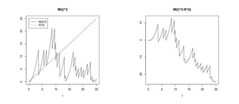
SimulatePoissonFigure1 — Figure 1: The resulting figures from Code 1, showing the sample paths of \(N(t)\) and \(M(t)\).

Code 2 shows code that adds a plot of the sample path of \(M^2(t)\) together with \(\lambda t\), and a plot of the sample path of \(M^2(t)-\lambda t\).

Kopier

plot(t,Mt^2,type="l",ylab="",ylim=c(0,max_time),main="M(t)^2")
lines(t,lambda*t,col="blue",lty=2)
legend(0,max_time,c("M(t)^2","N*(t)"),col=c("black","blue"),lty=c(1,2))


plot(t,Mt^2-lambda*t,type="l",ylab="",main="M(t)^2-N*(t)")

Code 2: Adding plots for \(M^2(t)\).

Figure 2 shows these plots.

SimulatePoissonFigure2 — Figure 2: The resulting figures from Code 2, showing the sample paths of \(M^2(t)\) and \(M^2(t)-\lambda t\).